RAG Done Right: A Practical Architecture Guide for Real-World Enterprise Systems
2025-11-30 • Generative-AI,AI,RAG,LLMs • Sam Madireddy
Retrieval-Augmented Generation (RAG) is now the backbone of many enterprise AI systems — from copilots to knowledge assistants to internal engineering tools. But although most organizations are rushing to adopt RAG, very few succeed in making it reliable, scalable, and production-ready.

RAG doesn’t typically fail because of the LLM. RAG fails in most cases because retrieval is broken.
In this article we’ll walk through how to design RAG the right way, using patterns that actually hold up in real systems. We’ll look at:
👉 Why RAG Fails in Real Enterprise Systems
👉 The eight pillars of RAG architecture
👉 Python snippets for embeddings and retrieval
👉 AWS patterns using Bedrock, Lambda, S3, and OpenSearch
👉 Retrieval quality techniques (hybrid search, RRF, re-ranking)
👉 Observability, latency, and cost-management strategies
1. Why RAG Fails in Real Enterprise Systems
1.1 Poor chunking strategies
Most real-world RAG failures begin right at the chunking layer. Teams either make chunks far too large or far too small, and both mistakes quietly break retrieval long before the LLM sees anything.
Chunks that are too large
Symptoms
- Chunks are 1,500–3,000 tokens because “the model has a large context window”.
- Retrieval returns a few massive passages where most content is irrelevant.
- LLM responses become either vague (“it depends…”) or confidently mix unrelated parts of the document.
Why this breaks things
- Embeddings represent the average meaning of the chunk, so local details get washed out.
- A chunk that discusses 10 topics dilutes the specific part the user cares about.
- Reranking struggles because every candidate is noisy.
Chunks that are too small
Symptoms
- Chunks are 1–2 sentences, or ~100–150 characters.
- The index explodes into millions of tiny vectors.
- Retrieval returns many isolated snippets that look relevant in isolation but lack context.
Why this breaks things
- You lose local structure: lists, tables, definitions, headings, examples.
- Pronouns and references (“it”, “above”, “this requirement”) point outside the chunk.
- The LLM has to stitch together dozens of fragments, which increases confusion and cost.
🎯 Why this matters
If chunking is wrong, no amount of clever embeddings, reranking, or prompting will save you. The model can only reason over the pieces of text it’s given.
What you should implement
- For typical enterprise docs, aim for 500–800 tokens per chunk.
- Use a semantic or heading-aware chunker where possible (respect sections, headings, bullets).
- Keep a small overlap between neighboring chunks (15–25%) so context flows naturally.
- Avoid breaking tables, bullet lists, or sentences in the middle.
Getting chunking roughly right up front dramatically increases the chance that retrieval returns the right pieces of context instead of random fragments.
1.2 Weak metadata
Metadata is what tells your RAG system where a chunk of context came from and how it should be used.
Without useful metadata — such as domain, timestamp, system, author, or tags — retrieval becomes random and nearly impossible to debug.
🎯 Why this matters
When your user asks “Why did I get this answer?”, you want to explain it in terms of which document, which system, and which version was used.
A simple example for a chunk might look like this:
{
  "domain": "ops-knowledge-base",
  "timestamp": "2024-08-17T10:15:00Z",
  "system": "inventory-management",
  "author": "KnowledgeBase v3",
  "tags": ["policies", "operations"]
}
With this metadata in place you can:
- Filter to only the latest version of a document.
- Restrict retrieval to a given domain (for example, “pricing” vs “operations”).
- Debug relevance issues by checking which system and timestamp produced a bad chunk.
1.3 Choosing the wrong vector database
Another common failure mode is picking a vector store based on what already exists in the environment (“we already have X, so we’ll just use it”) instead of how the retrieval system needs to behave.
🎯 Why this matters
Vector search has very different requirements from OLTP or generic logging workloads. Latency, recall, filtering, and scaling patterns all depend on the store you choose.
Overkill for small systems
For small RAG systems (tens of thousands of docs), using a heavy distributed vector database can be unnecessary:
- You pay for cluster management, replicas, and network hops.
- Latency can actually be worse because of over-distribution.
- Operational overhead (snapshots, failover, index warm-up) adds complexity you don’t need.
Too small for growing workloads
On the other end, pushing millions of embeddings into a single-node store (like a small Postgres with pgvector or a local FAISS index) will eventually hit:
- Slow queries as the index grows.
- Increased timeouts under load.
- Painful reindexing and maintenance windows.
Simple rule of thumb
Use a scale-based guideline:
| Scale | Good options | Notes |
|---|---|---|
| Small (≤ 100K docs) | SQLite / local FAISS / light pgvector | Great for prototypes and low-volume tools. |
| Medium (100K–10M vectors) | Postgres + pgvector, Qdrant, Milvus | Balance of flexibility, filters, and performance. |
| Large (10M+ vectors or high QPS) | Pinecone, Weaviate, Amazon OpenSearch k-NN / Aurora VE | Designed for horizontal scaling, streaming ingestion, and high recall. |
Choosing the right class of vector store early makes retrieval behavior much more predictable as your RAG system grows.
1.4 Latency and cost surprises
Even with a solid architecture, RAG systems can become slow and expensive over time.
- Embedding large documents repeatedly instead of precomputing embeddings.
- Using unnecessarily large LLMs for every request.
- Over-provisioned or poorly tuned OpenSearch clusters.
- Context windows that always hit the maximum token limit.
🎯 Why this matters
If you don’t design with latency and cost in mind, your system may technically “work” but be unusable in production.
What you should implement:
- Precompute embeddings during ingestion; do not embed on every user query.
- Choose smaller embedding models by default and justify upgrades only when needed.
- Implement chunk- and query-level caching (for example, in DynamoDB or Redis).
- Cap the number of retrieved chunks and enforce a context token budget.
- Track p95 and p99 latency for every major hop: API Gateway, Lambda, vector store, and LLM call.
- Tune or right-size OpenSearch clusters instead of letting them grow unchecked.
1.5 No observability
When observability is missing, your RAG system becomes a black box:
- You don’t know why answers get worse over time.
- You can’t measure hallucinations or grounding failures.
- Latency and cost regress without warning.
- Retrieval drift goes undetected.
🎯 Why this matters
You can’t improve what you cannot see. A production RAG system must expose metrics and traces from day one.
A practical baseline is to log, per query:
- Retrieval hit rate (did we find any relevant chunks at all?)
- Average relevance score of the top-k results.
- Diversity of sources and documents in the top-k.
- Token usage (prompt + completion) per call.
- Latency broken down by retrieval and generation.
- User feedback (thumbs-up/down, explicit ratings, error reports).
Store this in DynamoDB or a logging system, and build CloudWatch dashboards or Grafana panels that let you watch these metrics over time.
2. The Eight Pillars of Production-Grade RAG
2.1 Document preprocessing
Before you even think about embeddings, you want clean, well-structured text.
That means:
- removing boilerplate (headers, footers, navigation),
- collapsing duplicates,
- respecting semantic boundaries like headings and sections.
The goal is to present the embedding model with coherent chunks that each “say one thing well”.
🎯 Why this matters
If your input is noisy, your embeddings will be noisy, and retrieval quality will drop regardless of model size.
One simple, heading-aware chunker might look like this:
export function chunkWithHeadings(text: string): string[] {
  const chunks: string[] = [];
  let current = "";
  for (const line of text.split("\n")) {
    if (line.trim().startsWith("#")) {
      if (current) chunks.push(current);
      current = line + "\n";
    } else {
      current += line + "\n";
    }
  }
  if (current) chunks.push(current);
  return chunks;
}
2.2 Embedding strategy
Choosing the right embedding model — and using it consistently — is one of the biggest levers you have for RAG quality. Many retrieval issues trace back to the embedding layer, not the LLM.
What teams often get wrong
- Using a general-purpose LLM as the embedding model: slow, expensive, and not tuned for retrieval.
- Picking an embedding model that doesn’t match the domain (for example, generic text for very structured SOPs).
- Re-embedding the entire corpus every time chunking or preprocessing changes.
Embedding stability matters just as much as embedding accuracy.
Simple, AWS-friendly model choices
You don’t need a huge menu of options. In practice, a few models cover most enterprise workloads:
| Data type | Recommended model | Why |
|---|---|---|
| General enterprise text | Amazon Bedrock Titan Embeddings G1 – Text | AWS-native, scalable, strong default for mixed content. |
| Technical / structured docs | E5-base (open source) | Better for procedures, APIs, and engineering docs. |
| Multilingual content | bge-m3 | Good cross-language semantic consistency. |
If you want one safe default on AWS, start with Titan Embeddings G1 and only switch when you have clear evaluation results that justify it.
Keep the pipeline consistent
Regardless of which model you choose:
- Normalize case, whitespace, and Unicode the same way everywhere.
- L2-normalize embeddings (unless your vector DB does it automatically).
- Version your embedding model and chunking strategy so you know which vectors came from which configuration.
A stable, well-documented embedding pipeline makes retrieval behavior much easier to reason about.
Example: embedding and storing documents
from sentence_transformers import SentenceTransformer
import numpy as np

model = SentenceTransformer("intfloat/e5-large")  # or call Amazon Titan Embeddings via Bedrock

documents = [
    "Refund policy for international flights depends on fare class and region.",
    "To reset your corporate VPN token, contact service desk with your employee ID.",
    "AWS Kendra frequently becomes expensive without document-level access controls.",
]

embeddings = model.encode(documents, normalize_embeddings=True)

print("Embeddings shape:", np.array(embeddings).shape)
from qdrant_client import QdrantClient, models

client = QdrantClient(":memory:")

client.recreate_collection(
    collection_name="enterprise_docs",
    vectors_config=models.VectorParams(
        size=len(embeddings[0]),
        distance=models.Distance.COSINE,
    ),
)

client.upload_collection(
    collection_name="enterprise_docs",
    ids=[1, 2, 3],
    vectors=embeddings,
    payloads=[
        {"text": documents[0], "category": "refund_policy"},
        {"text": documents[1], "category": "it_support"},
        {"text": documents[2], "category": "aws_costs"},
    ],
)
query = "How do I reset my VPN token?"
query_emb = model.encode(query, normalize_embeddings=True)

results = client.search(
    collection_name="enterprise_docs",
    query_vector=query_emb,
    limit=3,
)

for r in results:
    print(r.payload["text"], "(score:", r.score, ")")
This pattern keeps your embedding strategy simple, AWS-aligned, and easy to evolve as you evaluate models.
2.3 Vector store selection
A well-chosen vector store determines latency, recall, and scalability. At enterprise scale, you want predictable performance under load, good metadata filtering, and stable ingestion pipelines. Your choice also affects cost—distributed stores shine at high volume, while simpler stores are more suitable for compact corpora.
- OpenSearch for hybrid search (BM25 + vector + filters).
- Aurora PostgreSQL with pgvector when you want SQL and tighter control.
2.4 Retrieval logic
A strong retrieval pipeline blends the strengths of both lexical search and vector search.
BM25 (lexical) is excellent at matching exact terms and phrases. Vector search captures meaning and semantic similarity, even when the wording is different. Both are valuable — and neither is enough on its own for real enterprise content.
In a production RAG system, you typically:
-
Run a lexical search (BM25) over your indexed text.
Great at handling exact matches, terminology, error codes, product names, and acronyms. -
Run a vector search over your embeddings.
Pulls in semantically similar passages even when the query phrasing changes. -
Fuse the two result sets using a ranking strategy such as Reciprocal Rank Fusion (RRF).
RRF gives you a stable, signal-rich ranking without needing complex weighting. -
Optionally apply an LLM-based re-ranker on the top candidates for even better ordering.
🎯 Why this matters
This hybrid approach gives you:
- The precision of keyword search
- The flexibility of semantic search
- Better recall-at-K across diverse enterprise documents
- Protection against one retrieval mode silently failing
Hybrid retrieval is one of the highest-impact improvements you can make to RAG quality, and it doesn’t require any model fine-tuning — just a better retrieval pipeline.
2.5 Reranking
Even after hybrid retrieval, you still end up with 5–50 candidate chunks. Not all of them should go into the LLM prompt. This is where reranking makes a big difference.
What reranking does
- Boosts chunks that are truly relevant to the query intent, not just keyword overlap
- De-emphasizes noisy or near-duplicate passages
- Improves the chance that the top 3–5 chunks actually contain the answer
In practice, you usually:
- Take the top N candidates from hybrid retrieval (for example, 30–50).
- Pass each
(query, chunk)pair through a cross-encoder reranker such as an E5 rerank model or an AWS-native option like Amazon Bedrock Titan Rerank. - Sort by reranker score and keep the top K (for example, 5–15) as your final context candidates.
When you can’t afford a full cross-encoder, you can approximate reranking by combining:
- Semantic score (vector similarity)
- Lexical overlap
- Metadata boosts (e.g.,
priority=high,document_type=runbook)
🎯 Why this matters
Reranking is a cheap step that greatly increases the odds that:
- The best chunks appear first
- The model sees grounded, high-signal context
- You pass fewer irrelevant chunks into the prompt
It often gives you more benefit than trying a “bigger” LLM.
2.6 Context assembly
Once you’ve reranked your chunks, you still need to build a clean context window that the LLM can consume. This is more than just concatenating text.
A strong context assembly pipeline will:
- Deduplicate overlapping content so the model isn’t reading the same thing multiple times.
- Sort by relevance so the most important information appears first in the prompt.
- Enforce a token budget so you stay within latency and cost limits (for example, 1–2K tokens for most Q&A flows).
- Preserve some structure — headings, bullet lists, and section labels — so the model can see topic boundaries.
- Optionally group chunks by document or section so the answer can reference a specific source cleanly.
You can think of this step as building a mini “context document” on the fly: coherent, de-duplicated, and ordered.
🎯 Why this matters
Even perfect retrieval fails if the model sees a noisy, repetitive, or badly ordered blob of text. Clean context assembly is the “last mile” of RAG and directly affects grounding quality, hallucination rate, and token usage.
2.7 Generation layer
Once you have a ranked, de-duplicated set of chunks, you need to turn them into a prompt that the LLM can actually work with.
This step is more than just concatenating text:
- Deduplicate chunks so the model is not reading the same content multiple times.
- Sort by relevance so the most important information appears first.
- Enforce a token budget so you stay within latency and cost limits.
- Preserve some structure (headings, bullet lists) to help the model see topic boundaries.
- Make the instructions explicit: how to answer, what not to do, how to cite sources, and how to handle uncertainty.
🎯 Why this matters
The LLM can only reason over what it sees in the prompt. A clean, focused context window and clear instructions lead to better grounding, fewer hallucinations, and predictable token usage.
2.8 Observability & guardrails
You can’t improve what you can’t see.
Track:
- Cost (per request and per feature)
- Latency (end-to-end and per component: retrieval, reranking, generation)
- Relevance (eval Q&A pairs, human feedback, click data)
- Hallucination rate (how often the answer cites content that isn’t in context)
- Retrieval drift (when top chunks stop containing ground truth sections as the corpus evolves)
Enforce guardrails such as:
- Maximum chunk counts
- Minimum relevance scores
- Required citations or evidence snippets
- Fallback behavior when retrieval fails (e.g., “I don’t know based on the available documents.”)
Good observability turns RAG from a one-off prototype into a system you can confidently operate in production.
3. AWS Enterprise RAG Architecture
Designing a RAG system on AWS is easier when you split it into three clear paths: Ingestion, Inference, and Observability. Each path has a specific responsibility and can be scaled or tuned independently.
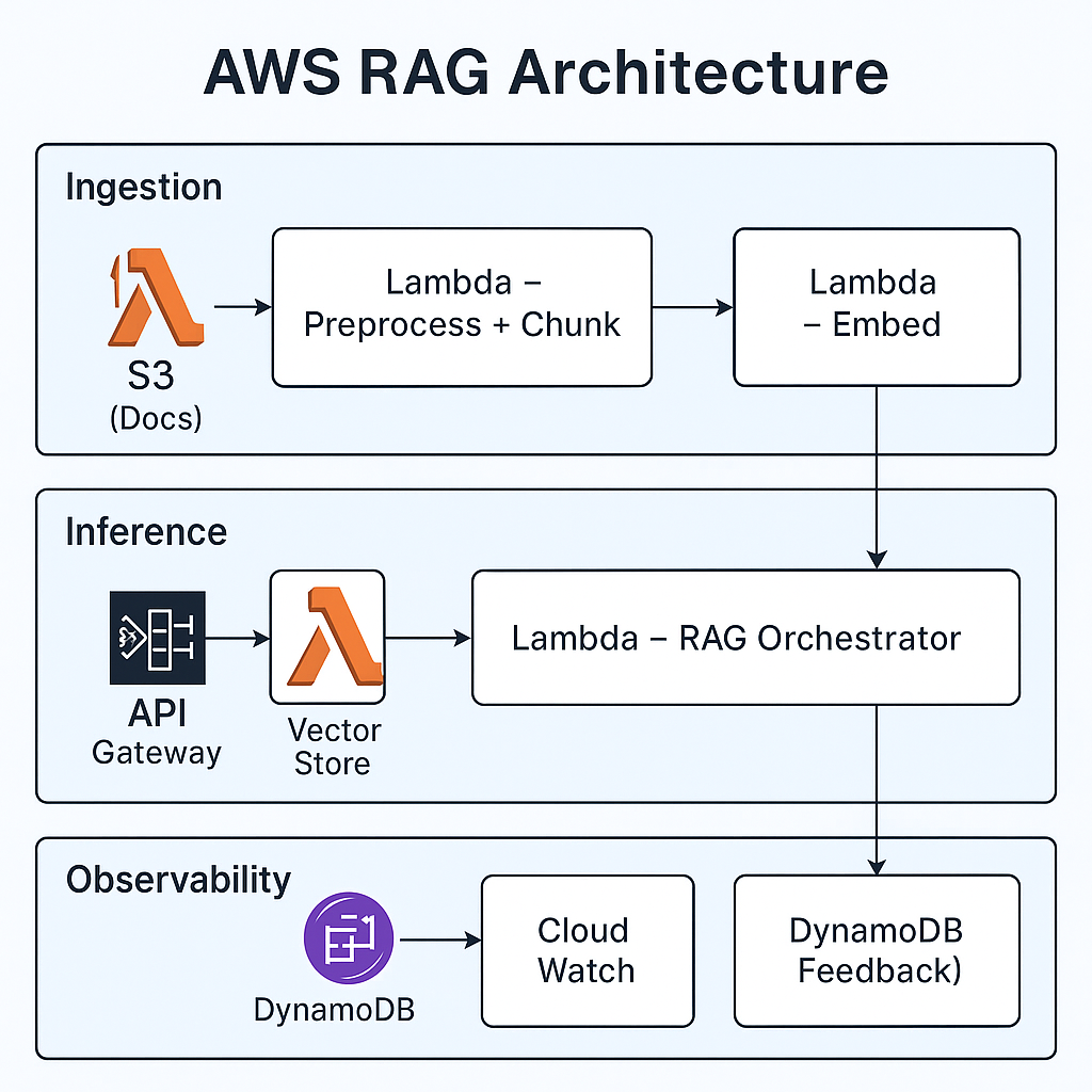
Ingestion pipeline (offline / async)
The ingestion pipeline prepares all documents before they are ever used to answer a query:
- S3 stores raw documents such as PDFs, DOCX files, HTML exports, and logs.
- A Lambda function performs preprocessing and chunking — cleaning text, extracting sections, and generating semantic chunks.
- Another Lambda function calls the embedding model and generates embeddings for each chunk.
- A vector store (such as OpenSearch or Aurora PostgreSQL with pgvector) stores embeddings alongside the metadata discussed earlier.
The heavy work happens here, away from the user-facing path.
Inference pipeline (real-time)
When a user sends a query, the inference path is responsible for answering quickly:
- API Gateway receives the query from UI clients or other services.
- A Lambda “RAG orchestrator”:
- embeds the query,
- performs hybrid retrieval (lexical + vector),
- applies ranking and optional re-ranking,
- builds the final context,
- calls Bedrock to generate the answer.
- The orchestrator returns a grounded response plus optional source citations.
This pipeline is optimized for low latency and predictable cost.
Observability and feedback
To keep the system healthy over time, you need continuous observability:
- CloudWatch and X-Ray capture latency, errors, and traces across the ingestion and inference pipelines.
- A DynamoDB feedback store records user ratings, flags for bad answers, and additional metadata such as which documents were used.
🎯 Why this matters
RAG is not just “an LLM plus a vector database”. It is a full system with ingestion, retrieval, generation, and feedback loops. Treating these as first-class components on AWS gives you room to evolve the system without constant rewrites.
4. Architecture View: What Really Matters in RAG
When you look at RAG through both an architect and tech-lead lens, a few priorities stand out:
- Retrieval quality beats model size. If the wrong chunks are retrieved, no LLM can rescue the answer.
- Metadata modeling is a first-class design step. Domain, timestamp, system, customer/account identifiers, and document type should all be queryable.
- Hybrid search is the default, not an afterthought. Combine lexical (BM25) + vector similarity + filters; use fusion or re-ranking to get the final set.
- Cost and latency are architecture concerns. Design explicit budgets for tokens, embedding frequency, and OpenSearch/vector-DB sizing.
- Chunking should be simple and explainable. Reasonable heuristics (headings, sections, semantic boundaries) beat over-engineered pipelines.
- Observability is part of the system, not a dashboard later. Track retrieval hit-rate, relevance score, hallucination rate, and cost per query from day one.
- Build reusable retrieval utilities. Don’t let every team invent its own ad-hoc RAG pipeline; ship a shared retrieval + generation module others can call.
- Treat RAG as a product capability, not a prototype. Think versioning, rollout, evaluation windows, and feedback loops.
5. Putting It Together: A Simple RAG Pipeline
def rag_pipeline(query: str):
    """End-to-end RAG pipeline: embed → retrieve → build context → generate."""
    q_vec = embed(query)
    docs = rag_retrieve(query, q_vec)
    ctx = build_context(docs)
    answer = generate_with_bedrock(query, ctx)
    return {"answer": answer, "sources": docs}
RAG done right is less about “prompt magic” and more about solid engineering: search quality, metadata design, cloud architecture, and careful attention to cost and latency.
When those are in place, the LLM finally has a chance to shine.
If you’d like to bounce ideas about RAG, AWS, or modern cloud architecture, feel free to reach out:
Sam Madireddy
Contact me on Linkedin